Abstract

Scene-dependent adaptive compressive sensing (CS) has been a long pursuing goal that has huge potential to significantly improve the performance of CS. However, with no access to the ground truth, how to design the scene-dependent adaptive strategy is still an open problem. In this paper, a restricted isometry property (RIP) condition-based error-clamping is proposed, which could directly predict the reconstruction error, i.e. the difference between the current-stage reconstructed image and the ground truth image, and adaptively allocate more samples to regions with larger reconstruction error at the next sampling stage. Furthermore, we propose a CS reconstruction network composed of Progressively inverse transform and Alternating Bi-directional Multi-grid Network, named PiABM-Net, that could efficiently utilize the multi-scale information for reconstructing the target image. The effectiveness of the proposed adaptive and cascaded CS method is demonstrated with extensive quantitative and qualitative experiments, compared with the state-of-the-art CS algorithms.

Adaptive sampling and reconstruction

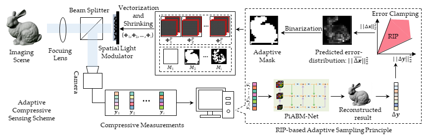
As shown in Fig. 2, different from the traditional CS model in Eq. 1, we propose an adaptive and cascaded multi-stage compressive sensing method, where the formulation of the $i$-th adaptive CS stage is \begin{equation} \label{eq:progressive} \begin{cases} \begin{aligned} &\boldsymbol{y}_{i} = \Phi_{i} \boldsymbol{x} + \boldsymbol{\epsilon_i},\\ & \hat{\boldsymbol{x}}_i = \mathcal{N}_{i}(\boldsymbol{y}_1, \boldsymbol{y}_2, ..., \boldsymbol{y}_i), \\ & \Phi_{i+1} = \mathcal{H}(\hat{\boldsymbol{x}}_i ), \end{aligned} \end{cases} \tag{1} \end{equation} where $\boldsymbol{x}$ is the target image, $\boldsymbol{y}_i$ is the measurement vector of the $i$-th stage. $\Phi_i$ denotes the corresponding sampling matrix, $\mathcal{N}_{i}(\cdot)$ indicates the reconstruction function from the set of previous measurements $\{\boldsymbol{y}_1, \boldsymbol{y}_2, ..., \boldsymbol{y}_i\}$ to the estimation of target image $\hat{\boldsymbol{x}_i}$ at the $i$-th stage. In this paper, $\mathcal{N}_{i}(\cdot)$ denotes the proposed PiABM-Net. $\mathcal{H}(\cdot)$ denotes the proposed adaptive module based on the RIP condition.

Figure 2. The diagram of the proposed multi-stage adaptive sampling scheme.

Error-induced Adaptive Module

According to the relationship between the sampling measurements and reconstructed results, we can calculate the measurements error $\Delta \boldsymbol{y}^{j}$ of image patch $j$ by \begin{equation} \Delta \boldsymbol{y}^{j} = \Phi^{p} \Delta \boldsymbol{x}^{j} = \Phi^p ( \boldsymbol{x}^{j} - \hat{ \boldsymbol{x}}^{j}) = \boldsymbol{y}^{j} - \Phi^p \hat{ \boldsymbol{x}}^{j}, \label{eq:calc_resid} \end{equation} where $\Phi^{p}$ is the measurement matrix of each patch. $\Delta \boldsymbol{y}^{j}$ can be regarded as the measurement of $\Delta \boldsymbol{x}^j$ with the measurement matrix $\Phi^{p}$. Similar to the CS problem, estimating $||\Delta \boldsymbol{x}^{j}||_2^2$ from the known $||\Delta \boldsymbol{y}^{j}||_2^2$ is ill-posed. However, if the measurement matrix $\Phi^{p}$ satisfies the RIP and the signal $\Delta \boldsymbol{x}^j$ is approximately sparse, the magnification of the reconstruction errors of patches could be clamped by the measurement errors with the inequality \begin{equation} \frac{||\Delta \boldsymbol{y}^{j}||_2^{2}}{(1+\delta)} \leq ||\Delta \boldsymbol{x}^{j}||_2^2 \leq \frac{||\Delta \boldsymbol{y}^{j}||_2^{2}}{(1-\delta)}, \end{equation} where $\delta$ is the RIP constant. RIP provides a double side clamping for the $l_2$ norm of the reconstruction errors $\Delta \boldsymbol{x}^j$. Therefore, it is reasonable to conclude that if the measurement error $||\Delta \boldsymbol{y}^j||_2 ^ 2$ is relatively large, the corresponding reconstruction error $||\Delta \boldsymbol{x}^j||_2 ^ 2$ is probably large as well, and vice versa. It is worth noting that for the traditional random measurement matrix, both $\Phi^p$ and $\Phi^p\Psi$ meet RIP well so that both the reconstruction of $\boldsymbol{x}$ and the prediction of $\Delta \boldsymbol{x}$ are well-defined. As for the learned measurement matrix, the RIP of $\Phi^p$ for prediction $\Delta \boldsymbol{x}$ is not guaranteed, so we impose an RIP loss on the measurement matrix $\Phi^p$ to provide a theoretical guarantee to support the reliability of the error prediction subproblem. The details of the error-based adaptive method are concluded in Alg. 1.

Algorithm 1. Error-based adaptive scheme $\mathcal{H}(\cdot)$.

PiABM-Net for CS reconstruction

Figure. 3 shows the model of the proposed Progressive-inverse and Alternatively Bidirectional Multigrid Network (PiABM-Net) for the CS reconstruction at each stage. Instead of transforming the measurements to the full-resolution image domain directly, we propose to progressively project the measurements to the image domain at multiscale levels with a progressive-inverse transform for deep image reconstruction. The transformation can be summarized as, \begin{equation} \begin{cases} \begin{aligned} & f_{\frac{H}{4}\times \frac{W}{4}} = \mathcal{R}(A\boldsymbol{y}), \\ & f_{\frac{H}{2}\times \frac{W}{2}} = \mathcal{U}_1(\mathcal{R}(A\boldsymbol{y})), \\ & f_{H\times W} =\mathcal{U}_2(\mathcal{U}_1(\mathcal{R}(A\boldsymbol{y}))), \end{aligned} \tag{2} \end{cases} \end{equation} where $f_{\rm height \times width}$ denotes features with ${\rm height \times width}$ sizes, $H$ and $W$ are the spatial size of the target image, $\boldsymbol{y}$ is the measurements, $A$ is the $1\times 1$ convolution layer which can be regarded as a linear projection, $\mathcal{R}$ is the rearrange operation, $\mathcal{U}_1$ and $\mathcal{U}_2$ are the learnable upsampling process composed of a dense residual block, a $1\times 1$ convolution layer and a pixel shuffle layer. With the progressive-inverse transform, the measurements can be projected to the full-resolution image in a progressive way and multi-scale features are generated as the input for the following alternatively bidirectional multigrid network.

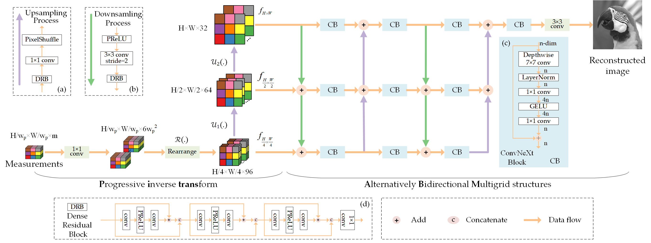
Figure 3. The overall structure of the proposed MGSANet. (a) The backbone of MGSANet, (b) upsampling module, (c) downsampling module, (d) Dense Residual Block, (e) Residual Block, and (f) Spatial Attention module.

Loss Function and Training Strategy

Given an input image $\boldsymbol{x}$ and the learnable measurement matrix $\Phi$, the sampling measurements can be denoted as $\Phi \boldsymbol{x}$. For network training, we adopt $l_1$ loss to supervise the reconstructed result as pixel loss: \begin{equation} \begin{aligned} \mathcal{L} ^\mathrm{pixel} = \|\mathcal{N}(\Phi \boldsymbol{x})-\boldsymbol{x}\|_1 , \label{eq:loss_pixel} \end{aligned} \tag{3} \end{equation} where $\mathcal{N}(.)$ denotes the reconstruction network. There are two RIP conditions should be satisfied in our scenario: 1) RIP on the sub-problem of signal sensing, through training the neural network for high accuracy signal recovery, the RIP condition with respect to $\Phi_c = \Phi \Psi$ could be satisfied; 2) RIP on the sub-problem of error prediction, we further impose an RIP loss to constrain the measurement matrix $\Phi^p$ to satisfy RIP. Given the measurement matrix of patches $\Phi^p \in R^{m\times n}$ with $l_2$-normalized columns $\phi_1,...,\phi_n$, where $n = w_p\times w_p$ is the pixel number of the patch and $w_p$ is the patch size. According to the Gershgorin circle theorem, RIP loss can be realized by constraining the sum of off-diagonal elements of each row of ${\Phi^p}^T \Phi^p$ to zero, that is: \begin{equation} \mathcal{L}^{\mathrm{RIP}} = ||{\Phi^p}^T \Phi^p-I||_1, \tag{4} \end{equation} where $I \in R ^ {n\times n}$ represents the identity matrix and the superscript $T$ represents the transposition of a matrix. We use RIP loss to minimize the lower and upper bounds by optimizing the near orthogonality of the measurement matrix $\Phi^p$ during the training process, the mathematical proofs are presented in Supp. The total loss function is the combination of the pixel loss and the RIP loss, \begin{equation} \begin{aligned} \mathcal{L} &= \mathcal{L} ^\mathrm{pixel}+\beta\ \mathcal{L}^\mathrm{RIP} \\ &= \|\mathcal{N}(\Phi \boldsymbol{x})-\boldsymbol{x}\|_1+\beta\|{\Phi^p}^T \Phi^p - I\|_1 , \label{eq:loss_func} \end{aligned} \tag{5} \end{equation} where $\beta$ denotes the loss-balancing hyper-parameter. For the multi-stage adaptive network training, we use Eq. 5 to train each CS sampling stage gradually. In other words, we train different stages separately by fixing the parameters of the previous stage after we complete the training process of the previous stage. Note that, for the input measurements, those patches that are not sampled in the adaptive sampling process are padded with 0.

Experiments

Quantitative results

we compare with the state-of-the-art CS algorithms proposed in recent years, i.e. AMP-Net, OPINE-Net+, COAST, NL-CS, MADUN and MS-CCSNet+. The quantitative comparison is shown in Tab. 1. As shown, the proposed AdaCS method outperforms the state-of-the-art CS methods in both PSNR and SSIM. Besides, we can see that the proposed method is more effective on image datasets with higher resolution, such as Manga109 and Urban100. That is because the sample number required for high-quality reconstruction of the patches usually possesses a larger variance in these high-resolution image datasets. Specifically, high-resolution images contain various image patches with very different contents, e.g., both smooth and textured regions, requiring quite different sampling rates for high-quality reconstruction. Benefiting from the adaptive allocation of the sampling rate, the proposed AdaCS network achieves much higher reconstruction quality at the same overall sampling rate.

Table 1. Performance comparison with SOTA CS algorithms on Set11, BSD68, BSDS500 testset, Urban100, OST300 and Manga109. The bold font is utilized to indicate the best results and the second-best results are marked with an underline.

Visual results

Figure 4 shows the visual reconstruction results, we can observe that the reconstruction results of our proposed method are closer to the ground truth and have clearer texture details. In all, through comparison with the SOTA methods, we demonstrate the superiority of our proposed method both quantitatively and qualitatively.

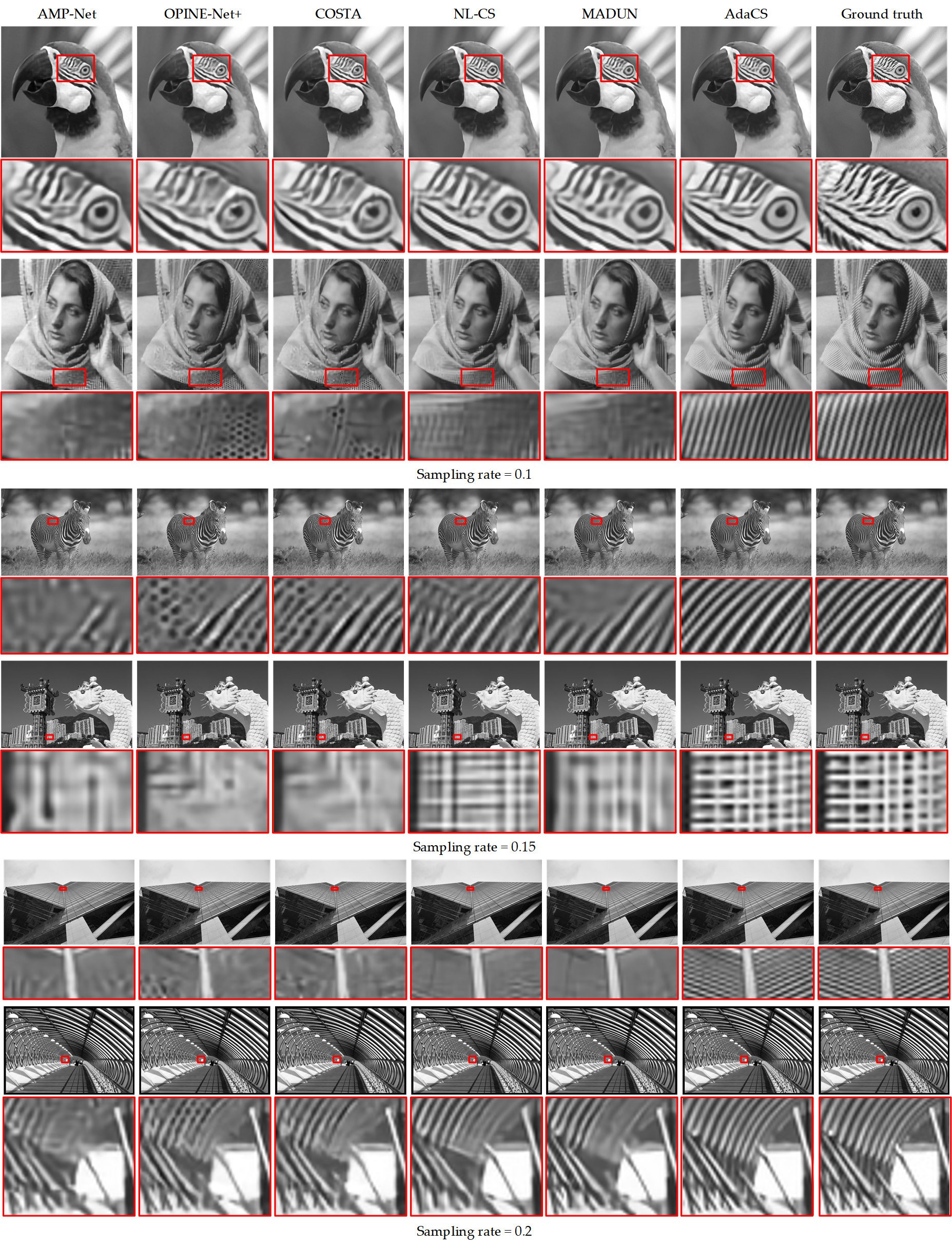
Figure 4. Visual comparison with the state-of-the-art CS algorithms.

More Details

• File
• Paper

Bibtex

@article{10412658,

author={Qiu, Chenxi and Hu, Xuemei},

journal={IEEE Transactions on Pattern Analysis and Machine Intelligence},

title={AdaCS: Adaptive Compressive Sensing with Restricted Isometry Property-Based Error-clamping},

year={2024},

volume={},

number={},

pages={1-18},

doi={10.1109/TPAMI.2024.3357704}}

}